
When Statistical Model Performance is Poor:
Try Something New, and Try It Again
Try Something New, and Try It Again
Bruce Ratner, Ph. D.
Typically, the data analyst approaches a problem directly with an (inflexible) procedure designed specifically for that purpose. For example, the everyday statistical problems of classification (i.e., assigning class membership with a categorical target variable), and prediction of a continuous target variable (e.g., sale or profit) are solved by the “old” standard binary or polynomial logistic regression (LR) models, and the ordinary least-squares regression (OLS) model, respectively. This is in stark contrast to the newer machine learning “algorithmic” methods, which are nominally statistical models, or more aptly non-statistical models, in that no effort is made to represent how the data were generated. There are nonparametric, assumption-free “flexible” procedures that let the data define the form of the model itself. The working assumption that today’s (big) data fit the OLS and LR models – which were formulated within the small-data setting of the day over 200 years ago, and 50 years ago, respectively – is not tenable. A flexible, any-size data model that is self-defining clearly offers a potential for building a reliable, highly predictive model, which was unimaginable two centuries ago, even a half century ago. The most notable algorithmic methods for the everyday statistical problems are the decision trees (sets of if-then rules), such as CART, CHAID, and C5.0.
To paraphrase, "Even the best-laid models go oft astray, and have poor performance." When a statistical model performance is poor: Try something new, an algorithmic method, which promises a better solution. Big data (and small data too!) bring the prospects of data complexity, namely, data points that are difficult to deal with, referred to as a "data mass," which renders initially poor model performance. Algorithmic methods are flexible, which implies they are resistant, yet are not immune to the hardest of data mass. To take on a data mass, do the following: 1) Apply the algorithmic method. 2) Retain the initial results (initial model), albeit the performance is wanting. 3) Reuse the initial model (as a new variable) by appending it into the original data. 4) Reapply the algorithmic method. 6) Repeat the previous tasks, as often as necessary, until model performance is worthy of being accepted. The purpose of this article is to present the algorithmic GenIQ Model©, a flexible, any-size data method that lets the data alone defines the model. I use the GenIQ Model in a real case study to show what to do when a model performance is poor.
Outline of Article
I. Situation
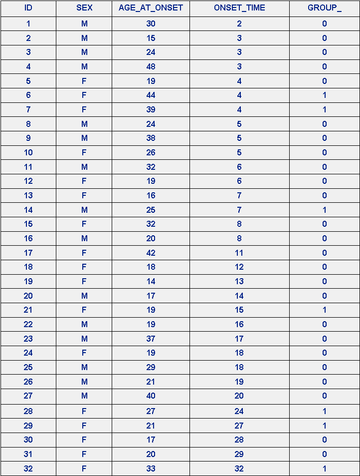
The data come from a study of multiple sclerosis (MS) – whether the disease is infectious. The possibility that the disease is infectious resides in the apparently sudden occurrence of MS in the Faroe Islands after British troops arrived there in 1941. There were two groups of patients: Those in Group A (coded GROUP_ = 0) had not been off the islands before onset, while those in Group B (coded GROUP_ = 1) had been off the islands for less than two years before the onset. Is there any evidence that MS is infectious? Effectively, if a model can be built to distinguish between the groups then the model is the evidence. The “MS" data are in Table 1, below (from Is multiple sclerosis an infectious disease? Biometrics, 46, 337-349).
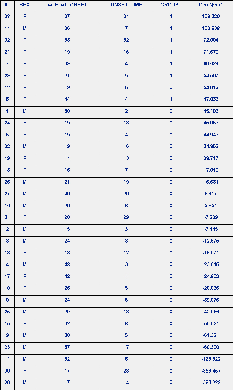
Table 1. MS Data
I built the easy-to-interpret logistic regression model (LRM), and the not-so-easy-to-interpret GenIQ Model for the target variable GROUP_.
II. LRM Output
The LRM output (Analysis of Maximum Likelihood Estimates) - arguably the best GROUP_-LRM equation (model) is:
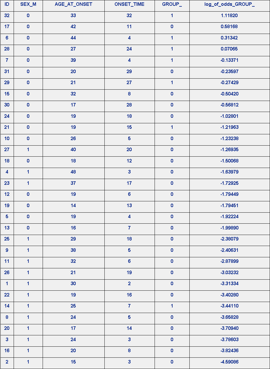
Log of odds of GROUP_(=1) = - 3.8768 + 2.2470*SEX_M + 0.0894*AGE_AT_ONSET + 0.0639*ONSET_TIME
where SEX_M=1 if SEX="M"; SEX_M=0 if SEX="F".
III. GROUP_-LRM Results
The results of the GROUP_-LRM are in Table 2. LRM log_of_odds_of_GROUP-Rank-order Prediction of GROUP_, below. There is not a perfect rank-order prediction of GROUP_. Patient ID #14 is consider the data mass, as it is poorly ranked #26.
Table 2. Rank-order Prediction of GROUP_ based on log_of_odds_of_GROUP_
IV. GenIQ Model Output
The GROUP_-GenIQ Model Tree Display and its Form (Computer Program) are below.
The GenIQ Model (Tree Display)
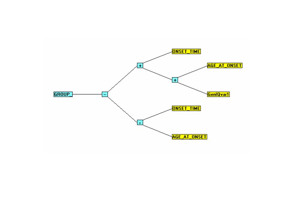
The GenIQ Model (Computer Program)
x1 = AGE_AT_ONSET;
x2 = ONSET_TIME;
If x1 NE 0 Then x1 = x2 / x1; Else x1 = 1;
x2 = GenIQvar1;
x3 = AGE_AT_ONSET;
x2 = x2 + x3;
x3 = ONSET_TIME;
x2 = x2 + x3;
x1 = x2 - x1;
GenIQvar = x1;
V. GROUP_-GenIQ Model Results
The results of the GROUP_-GenIQ Model are in Table 3. GenIQ Model GenIQvar Rank-order Prediction of GROUP_, below. There is a perfect rank-order prediction of GROUP_. Note as per the LRM, Patient ID #14, who was poorly ranked #26, is now reliably ranked #3.
Table 3. GenIQ Model GenIQvar Rank-order Prediction of GROUP_

VI. GROUP_-GenIQ GenIQvar1 Model Results
The GenIQvar1 Model (Tree Display)
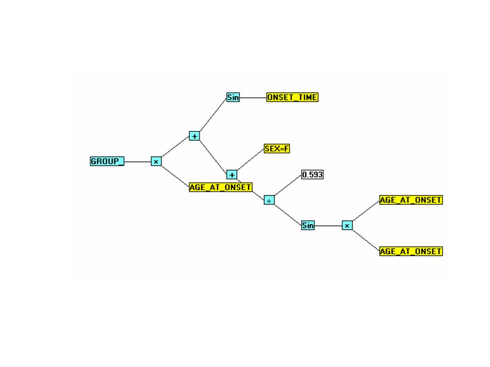
The GenIQvar1 Model (Computer Program)
x1 = AGE_AT_ONSET;
x2 = AGE_AT_ONSET;
x3 = AGE_AT_ONSET;
x2 = x2 * x3;
x2 = Sin(x2);
x3 = .5929195;
If x2 NE 0 Then x2 = x3 / x2; Else x2 = 1;
If SEX = "F" Then x3 = 1; Else x3 = 0;
x2 = x2 + x3;
x3 = ONSET_TIME;
x3 = Sin(x3);
x2 = x2 + x3;
x1 = x1 * x2;
GenIQvar1 = x1;
V. GROUP_-GenIQ GenIQvar1 Model Results
The results of the GROUP_-GenIQ GenIQvar1 Model are in Table 4. GenIQ Model GenIQvar1 Rank-order Prediction of GROUP_, below. There is not a perfect rank-order prediction of GROUP_. Patient ID #6 is consider the data mass, as it is misranked #8. Interestingly, as per the LRM, Patient ID #6 is not a data mass, as she is positioned in rank #3. Yet, as per the correct GenIQ GenIQvar Model, she is reliably placed at the end of the perfect ranking at position #7. As for Patient ID #14, who was poorly ranked by LRM in position #26, is ranked #2, and #3 by GenIQvar1 and the correct GenIQvar models, respectively.
Table 4. GenIQ Model GenIQvar1 Rank-order Prediction of GROUP_
IX.Summary
The machine learning paradigm (MLP) “let the data suggest the model” is a practical alternative to the statistical paradigm “fit the data to the equation,” which has its roots when data were only “small.” It was – and still is – reasonable to fit small data in a rigid parametric, assumption-filled model. However, today's big data require a paradigm shift. MLP is a utile approach for analysis and modeling big data, as big data can be difficult to fit in a specified model. Thus, MLP can function alongside the regnant statistical approach when the data – big or small – simply do not “fit.” However, when the best-laid statistical models go oft astray, and have poor performance, the approach is to try something new, and try it again.
Go to Articles page.
1 800 DM STAT-1, or e-mail at br@dmstat1.com.
574 Flanders Drive / North Woodmere, NY 11581 / U S A
Voice 1-516-791-3544 / Fax 1-516-791-5075
Toll Free 1 800 DM STAT-1